RL for Blackjack Part 3
Reproducing Thorp’s Basic Strategy
This is the third article in the ML for Blackjack strategy series. In the Part 2 I worked to reproduce the Monte Carlo with Exploring Starts Example 5.3 (Sutton and Barto 2020). I showed how policy iteration could be used to generate an optimal policy for blackjack that was nearly identical to the basic strategy calculated by Edward O. Thorp in the 1960s using combinatorial analysis. In this article I dig into why the policies where not exactly identical and expand the excercise to include additional actions and states.
Thorp’s Basic Strategy
The following tables represent the basic strategy for standing and hitting as reproduced from Beat the Dealer (Thorp 1966). Thorp produced these tables by painstakingly calculating the exact outcome probabilities from sampling without replacement from a single card deck.
Hard Hands
| You have | 2 | 3 | 4 | 5 | 6 | 7 | 8 | 9 | 10 | A |
|---|---|---|---|---|---|---|---|---|---|---|
| 17 | S | S | S | S | S | S | S | S | S | S |
| 16 | S | S | S | S | S | \(\ast\) | ||||
| 15 | S | S | S | S | S | |||||
| 14 | S | S | S | S | S | \(\dagger\) | ||||
| 13 | S | S | S | S | S | |||||
| 12 | S | S | S |
- \(\ast\) Holding hard 16: Draw if you hold two cards, namely (10,6) or (9,7), and stand if you hold three or more cards, for example, (6,4,4,2).
- \(\dagger\) Stand holding (7,7) against a 10
Soft Hands
| You have | 2 | 3 | 4 | 5 | 6 | 7 | 8 | 9 | 10 | A |
|---|---|---|---|---|---|---|---|---|---|---|
| 19 | S | S | S | S | S | S | S | S | S | S |
| 18 | S | S | S | S | S | S | S | S |
Reconciling with MC Results
In the previous article we produced a policy that was very similar to Thorp’s but with a few significant differences. First, as Sutton & Barto point out, Thorp’s strategy calls for standing on a soft 18 against a dealer ace while the previous results call for hitting a soft 18 against a dealer ace. Second, if you recall from the previous article, the difference between standing and hitting on a hard 16 against a dealer 10 was close to zero. But there are several ways to arrive at a hard 16, including two, three, and four-card combinations. In our MC simulations we collapsed the state so that all hard 16’s represented the same state. Thorp did not make this simplifying assumption and was able to refine those actions further (e.g. hit a \([10,6]\) but stand on a \([6,4,4,2]\)).
Single Deck or Infinite Deck
The first discrepancy is fairly easy to resolve. In Sutton & Barto’s example, they explicity state that an infinite deck is used.
We assume that the cards are dealt from an infinite deck (i.e. with replacement) so that there is no advantage to keeping track of the cards already dealt.
Thorp based his calculations on a single deck where cards are dealt without replacement. We can re-run our MC ES episodes using a more realistic deck model that keeps track of which cards have already been dealt.
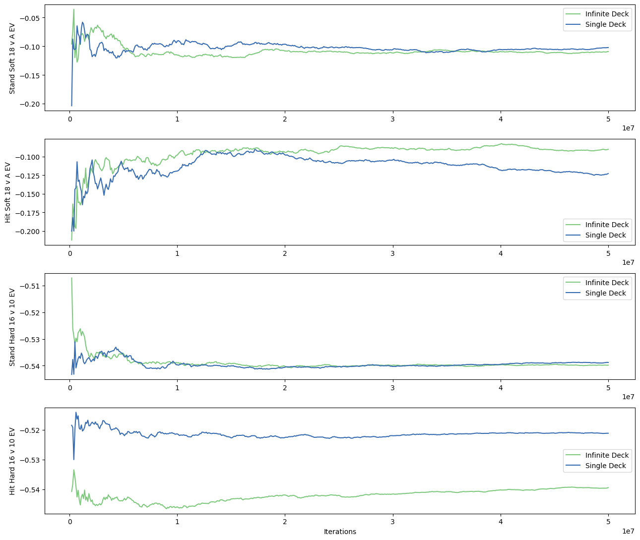
In Figure 1 we can clearly see a difference in the converged EV for hitting a soft 18 against a dealer ace. The EV when hitting in an infinite deck game is higher than hitting in a single deck game. This is enough to change the policy to stand for a single deck game. This explains the “notch” in the Sutton & Barto results for that particular state and reconciles the results with Thorp’s single deck calculations.
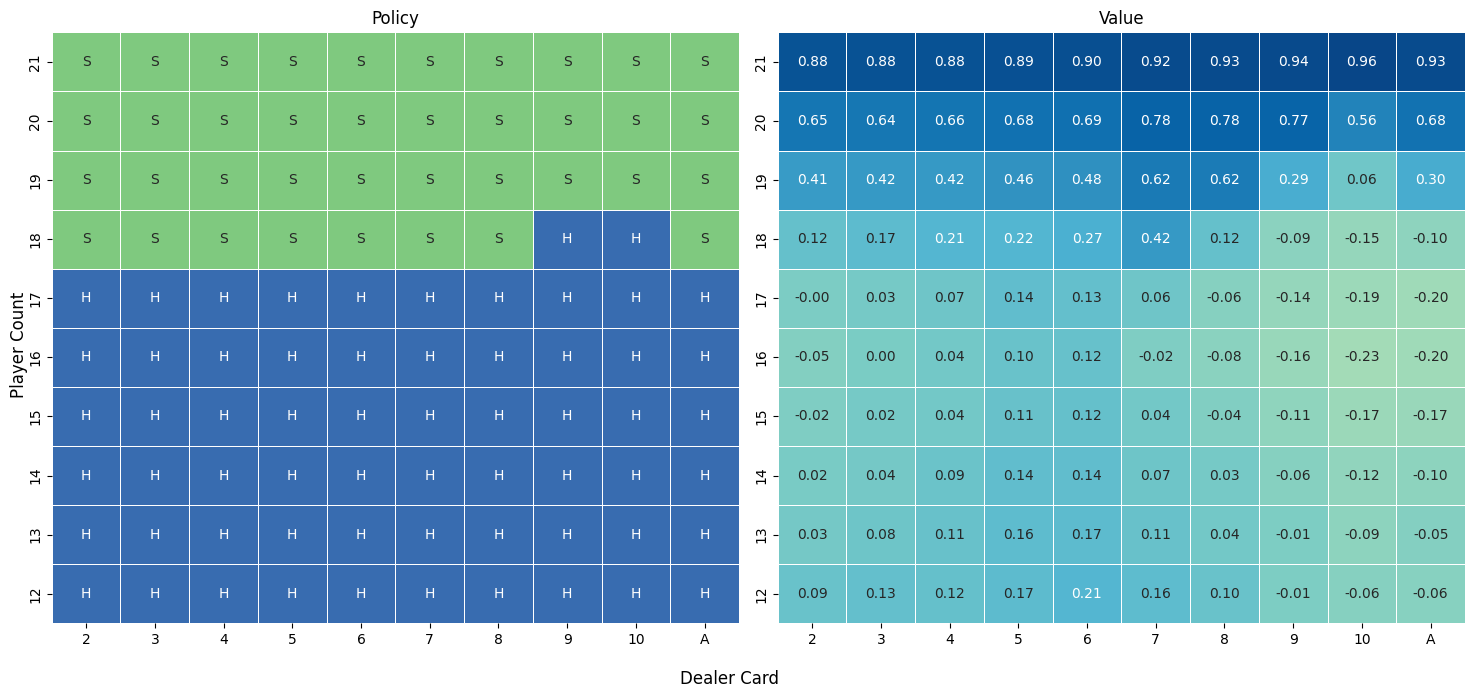
Multi-card Hands
In an infinite deck simulation, a 3-card 16 can be treated exactly the same as a 2-card or 4-card 16 because the probability of any next card is unchanged. This is not true for the single deck calculations that Thorp performed. Thorp also distinguished between some two card combinations that are a pair (e.g. \([7,7]\) and \([6,8]\) are both hard 14, but treated differently). This is partly because most blackjack games allow the player to split pairs and play them as two new hands. But it’s also related to the probability of winning a hand such as a \([7,7]\) where the best third card is a 7 but two of the 4 sevens are already depleted from the deck, reducing the chances of drawing the third 7 as the next card.
It’s possible to modify our state representation to account for the number of cards and whether we have a 2-card pair. Our initial state representation as suggested by Sutton & Barto was a 3-tuple of (player count, dealer card, useable ace). We can expand this representation into a 5-tuple of (player count, dealer card, useable ace, num player cards, player pair).
player count: value of all the cards in the player handdealter card: value of the dealer up carduseable ace: whether the player has an ace that is counted as 11 in his handnum player cards: number of cards in the player handplayer pair: whether the first two player cards are a pair
As an example, our previous state representation includes \((14,10,0)\), which is a hard 14 from any number of cards. In the new representation, this expands to the following:
- \((14,10,0,2,1)\) : \([7,7]\) versus a \([10]\).
- \((14,10,0,2,0)\) : \([6,8]\), \([5,9]\), or \([4,10]\) versus a \([10]\).
- \((14,10,0,3,0)\) : any 3-card 14 such as a \([2,2,10]\) versus a \([10]\).
- \((14,10,0,4,0)\) : any 4-card (or more) 14 such as a \([2,2,2,8]\) versus a \([10]\).
Obviously this increases the size of the state space. For practical reasons, I limited tracking the number of player cards to 4. So all hands with 4 or more cards summing to the same value represent the same state. Fortunately the size of the state space is still very manageable, increasing from 200 to 818.
Exploring Starts
By including the number of cards in the player’s hand we do introduce a tricky nuance as it relates to exploring starts. In order for MC ES to converge to an ideal policy, we have to guarantee that every state-action pair is explored appropriately. With the 3-tuple state space it’s fairly easy to do this just by repeatedly shuffling the deck, dealing cards, and randomizing the first action. Every state tracked by the 3-tuple state can be created from two cards plus a dealer up card. If we randomize the first action and then use the greedy policy to finish the game, we will over time still explore every state-action pair just by playing normal games.
However, by including 3 and 4-card hands in the state, we can no longer guarantee exploring starts just by playing games with a random first action and following a greedy policy thereafter. Consider an example where we initialize the policy to S on every hand and the player is dealt a \([5,6]\) against a \([5]\). This is state \((11,5,0)\) as a 3-tuple or \((11,5,0,2,0)\) as a 5-tuple. We randomly select the action H and the player draws a \([5]\) to give the hand \([5,6,5]\). This is now state \((16,5,0)\) as a 3-tuple or \((16,5,0,3,0)\) as a 5-tuple. The greedy policy for each was initialized to S, so the player stands and the dealer draws. Based on the outcome of the game we can update the value for the state-action pairs along the episdoe, \((11,5,0)\)-H or \((11,5,0,2,0)\)-H and \((16,5,0)\)-S or \((16,5,0,3,0)\)-S. The key difference is, on a subsequent exploring start, the game may start with the second state in the 3-tuple variation from a 2-card combo (e.g. \([6,10]\)). In this case the randomly selected action could be H instead of S so that the process will systematically explore both actions for that state in the normal course of dealing and playing blackjack. However, the 5-tuple state \((16,5,0,3,0)\) will never be reached as the first state by randomly dealing two cards for the player so the non-greedy action H will never be tested because a greedy policy is followed after the first random action.
There is more than one way to work around this problem. A commonly used strategy is to employ an \(\epsilon\)-greedy policy for the gameplay to ensure that more state-action pairs are explored. I chose to stick with exploring starts, which is possible by slightly modifying the starting hands in each simulated game. To satisfy the requirements for MC ES, we need to guarantee that every state-action pair in the 5-tuple state space is explored. To start we can generate every possible 2, 3, and 4 card player hand using a method like combinations_with_replacement. Here the choice of compressing every hand with 4 or more cards into a single state is useful because it means we do not have to worry about using more than 4 of a kind in the possible hand calculations. Also, not every 3 or 4 card combination is a valid starting hand in blackjack since the count of the cards must be less than or equal to 21. So from 2366 possible starting hands, we get 825 valid starting hands.
The next step is to determine the possible dealer up cards for each of the 825 valid starting hands. We can get those possible combinations by taking each valid starting hand, removing the player cards from the deck, and generating a combination of player hand and dealer up card from each remaining card in the deck. In this way we make sure that we don’t end up with impossible situations like a player hand of \([2,2,2,2]\) and a dealer up card of \([2]\) from a single deck shoe. After all this we get 10720 possible combinations of player hand and dealer up card for player hands up to and including 4 cards. This is still a very manageable number.
The final step is to modify the gameplay for the MC simulations to test all the possible states. Instead of randomly dealing cards we choose a random starting combination from the set of 10720 we generated. Then remove the cards that the player and dealer have in their hands from the deck, choose a random starting action, and then play the game as normal.
Policies for Expanded States
With these modifications we can get much closer to Thorp’s original results. Thorp’s Section 1.1 table shows two interesting exceptions against a dealer 10. In the first case, the policy says to hit a hard 16 if it’s a 2-card hand but stand otherwise. Using our expanded state we can look at both 2-card and 3+ card hard hands.
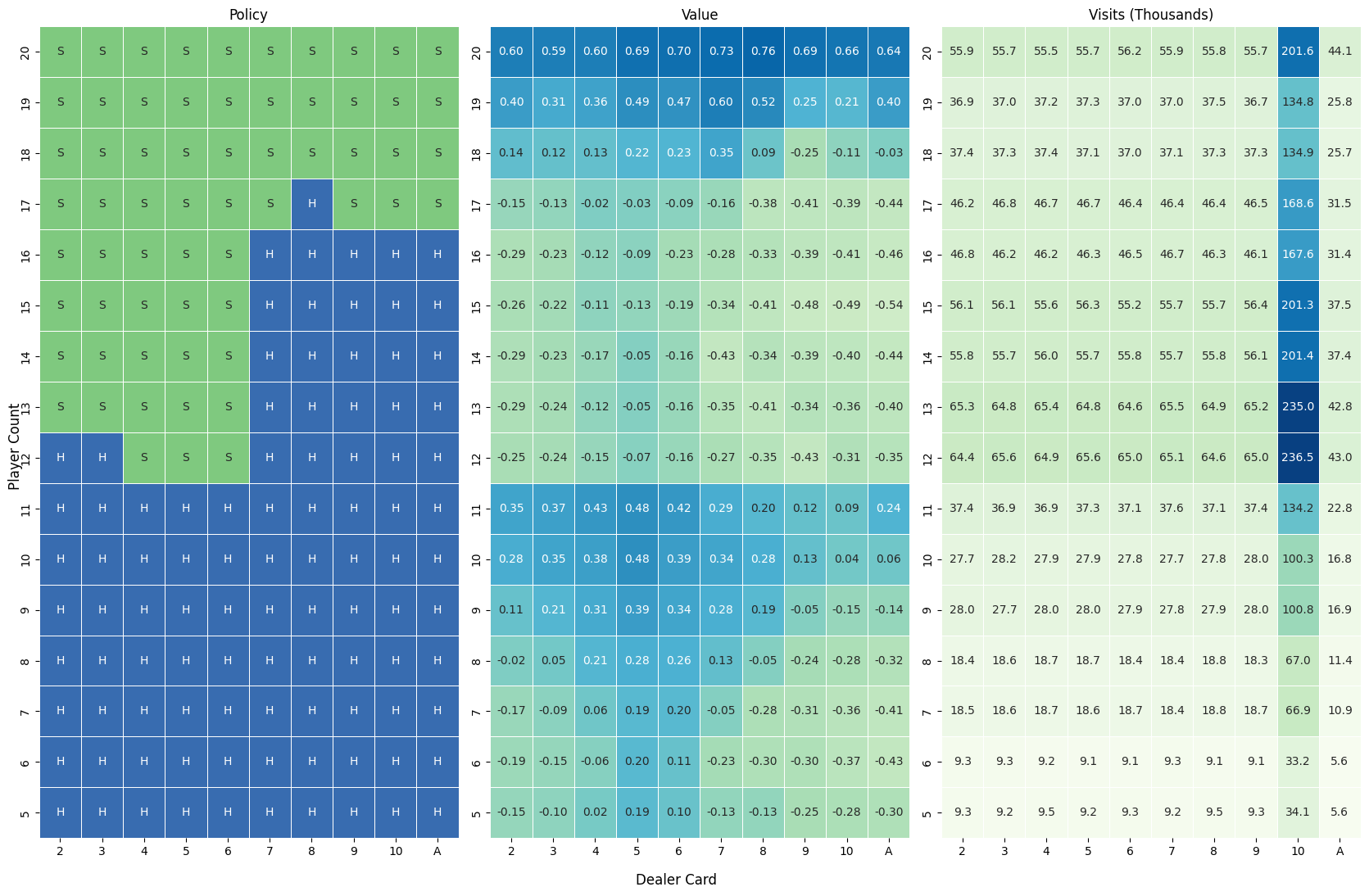
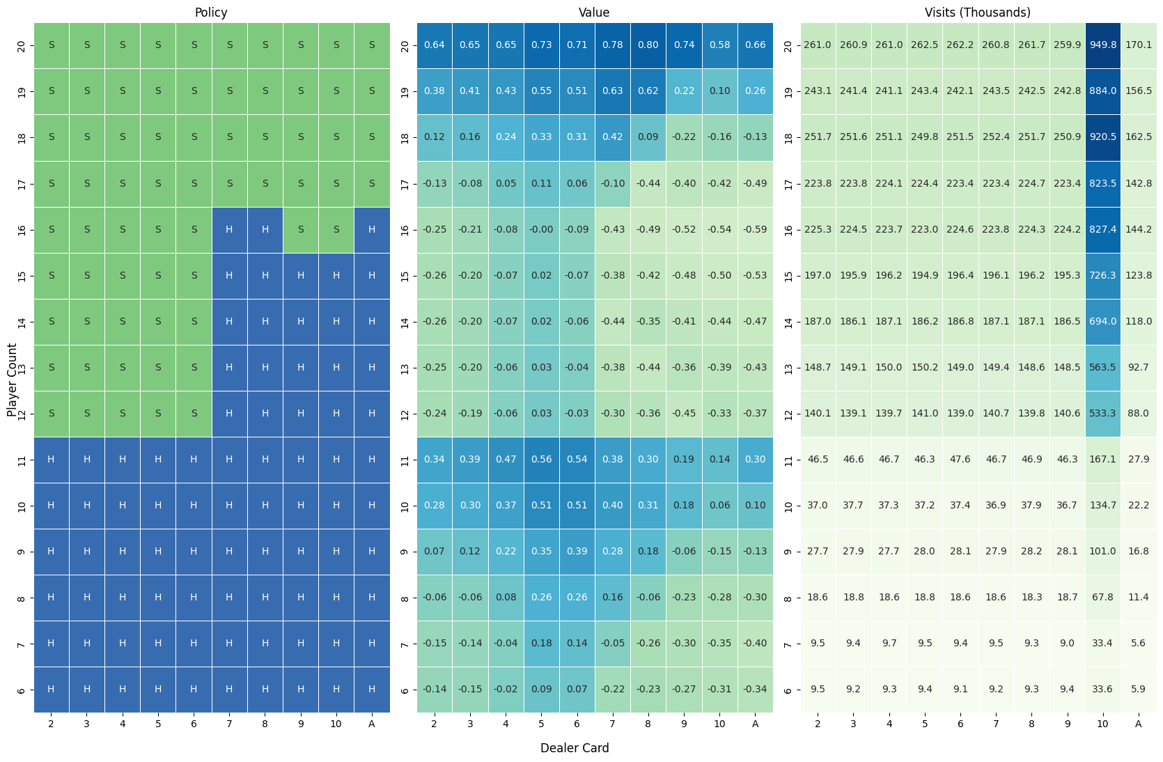
Comparing Figure 3 and Figure 4 does indeed show a difference in strategy between a 2-card 16 that is not a pair (e.g. \([6,10]\) or \([7,9]\)) and a 3-card 16, as suggested by Thorp. However, there are additional small differences for players holding hard 12, 16, or 17. It’s possible that Thorp didn’t include these as the regret from choosing one action over the other was so small that it wasn’t worth complicating the strategy.
For the second exception in Thorp’s Section 1.1 table, we need to look at strategy when holding a hard 2-card hand that is a pair. As predicted by Thorp, these results clearly show a carveout for standing with a \([7,7]\) against a dealer \([10]\).
Pair Splitting
It is important to note that this simulation did not include the possibility of splitting pairs. So the change in policy from hit to stand on \([7,7]\) against a dealer \([10]\) is purely due to the probability of winning the hand by taking a third card, not the ability to split and play two hands.
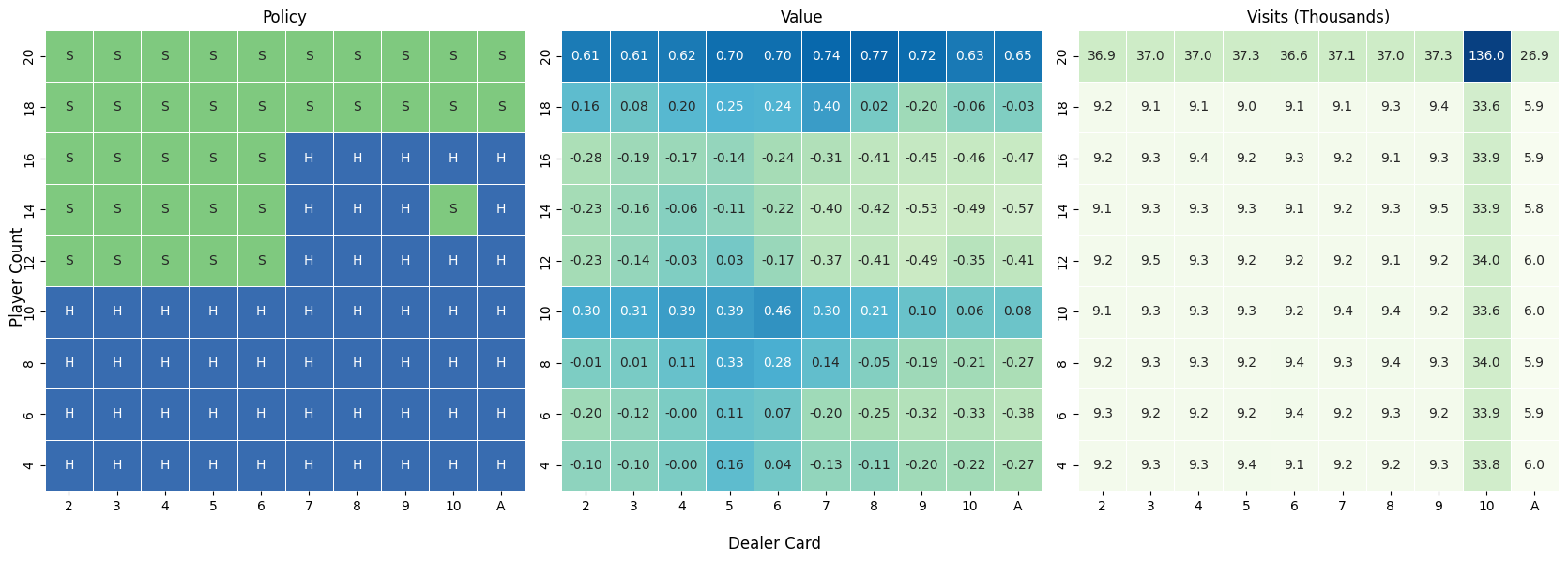
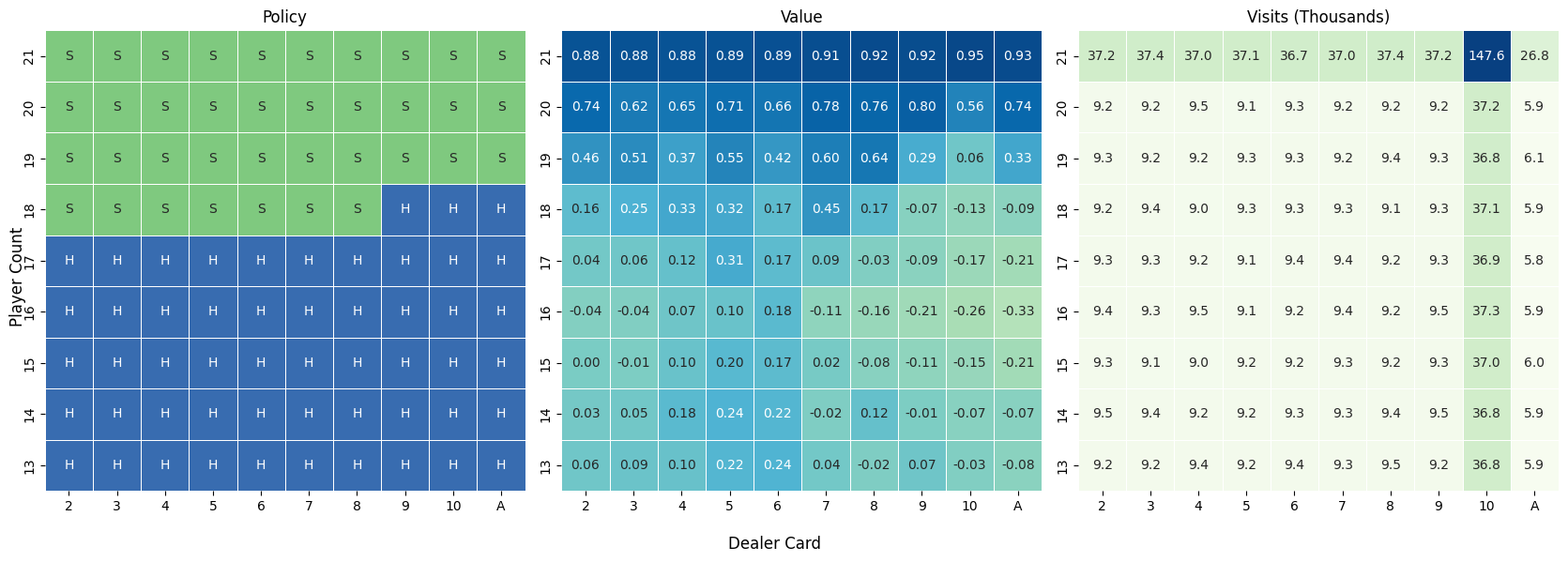
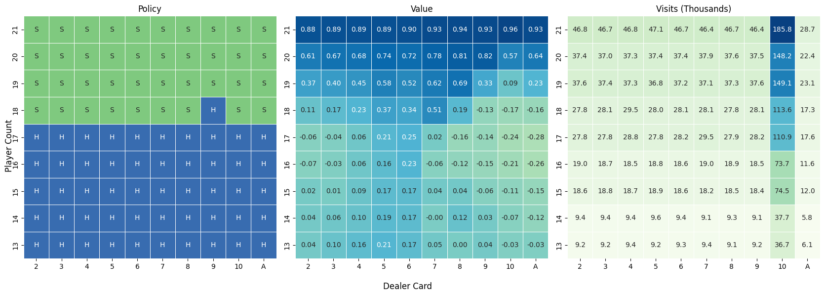
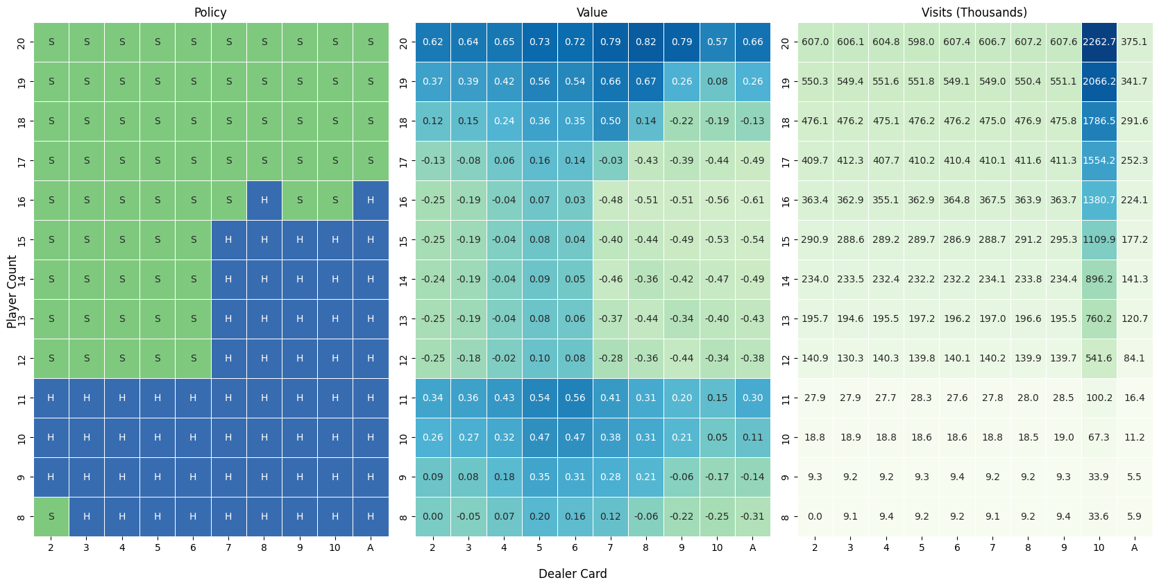
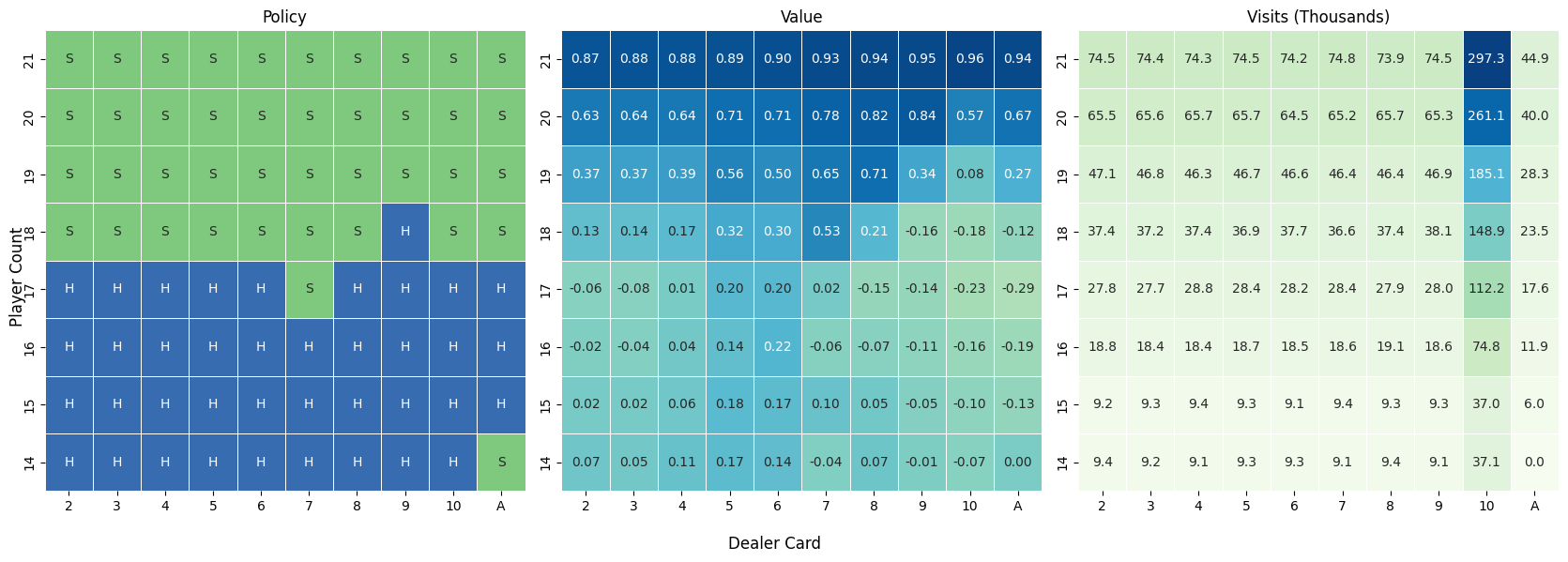
For completeness, I’ll show the generated policies for the remaining states. In general, the more cards in a player’s hand, the less likely the strategy is to hit instead of stand at values below 17.
Exploring Starts and Visits
In the policies for expanded states charts I also included the number of visits for each state. This was a useful tool to visually confirm that the criteria for exploring starts was being met. It’s also interesting to see that the number of visits to each state is not equal even though each state has the same probability of being chosen as a starting state. There are a few reasons for this. First, some states are more easily reachable through normal game play. For 3 or 4-card hands, the higher the player count, the more likely it is that the state will occur after starting as a 2-card hand. There are many more ways to make a 3-card 20 than a 3-card 6, for example. Second, there are 16 cards in each deck that have a value of 10. That means the probability of having at least one 10 in a 2-card hand is higher than the probability of any other card. Therefore there are many more visits to 2-card states with value 12 or greater than less than 12. Similarly, the probability of a dealer up card being a 10 is more likely than any other value, resulting in roughly 4 times as many visits to states with a dealer value of 10.