RL for Blackjack Part 2
Emulating Sutton & Barto
In Part 1 of this series I gave an overview of two different computational methods for coming up with an optimal strategy for the game of Blackjack. The first was a combinatorial analysis pioneered by Edward O. Thorp in the 1960s. The second is based on reinforcement learning approach described by Richard S. Sutton and Andrew Barto in Example 5.3 from their textbook. (Sutton and Barto 2020)
While Sutton & Barto don’t appear to have the same passion for beating casino games as Thorp did, they had at least enough interest to explore applying Monte Carlo policy iteration to a simplified version of blackjack.
Their simplifying assumptions are as follows:
- Player can only Hit or Stand (no doubling, splitting, or insurance)
- Dealer draws up to a value of 17 (some versions have the dealer hit on soft 17)
- The deck is sampled with replacement when a card is drawn (i.e. infinite deck)
The last point is of particular interest. With an infinite deck, the odds of drawing a specific card are always 1 in 52. In Thorp’s time, blackjack was often played with a single deck. As cards were dealt, the state of the deck changed, altering the probability of subsequent cards. In fact this became the entire basis of his later betting strategies that involved understanding how the remaining cards in the deck were likely to impact the player’s odds of winning.
Monte Carlo Exploring Starts
Monte Carlo Exploring Starts (MC ES) is a form of Monte Carlo control where the policy is improved iteratively after each episode. In MC ES, the requirement is that every state-action pair \((s, a)\) has a non-zero probability of being selected as the initial step of an episode. This “exploring start” ensures that the agent continues to gain experience with all possible trajectories, preventing the policy from prematurely converging on a suboptimal action simply because better alternatives were never sampled. By starting in every possible state and trying every possible action, the agent can accurately estimate the action-value function \(Q(s, a)\) for all pairs. Under these conditions, Sutton and Barto demonstrate that the policy can be updated “greedily” at the end of each episode (\(a = \arg\max Q(s, a)\)), eventually converging to the optimal policy \(\pi^*\) without the need for a stochastic policy (like \(\epsilon\)-greedy) during the learning process itself.
State Space
To come up with a strategy for blackjack we would like to have an optimal policy for every combination of cards a player might hold plus the single card that the dealer is showing. If we naively consider just the original two cards a player is dealt plus the dealer up card in an infinite deck, the total number of combinations is \(52^3 = 140608\). Fortunately in blackjack, the suits don’t matter and every face card is worth ten. This means we really just have ten values to track for state \([2, 3, 4, 5, 6, 7, 8, 9, 10, A]\). Also, order of the cards in a hand doesn’t matter. A \([10, 6]\) is worth the same as a \([6, 10]\).
To get the size of the state space, we can multiply the number of unique dealer hands by the number of unique player hands. We already know the number of unique dealer up cards is 10. For the number of player hands, we can use the formula for combination with replacement:
\[ \frac{n(n+1)}{2} = \frac{10 \times 11}{2} = 55 \]
This gives us \(10 \times 55 = 550\) possible starting states. However, this does not take into account the additional states that are generated as the player draws more cards. In addition, an ace can have a value of 1 or 11 depending on the count of the hand. If the player’s hand count is over 21 and the player has an ace that was valued as 11 to make the count, that ace takes a value of 1 to keep the player from busting. An ace that is counted as 11 is considered a “useable ace.”
Sutton & Barto point out that we can compress the state space quite a bit if we only consider the sum of the player’s cards. This means that the hands \([5,7]\), \([2,10]\), and \([4,5,3]\) are all equivalent since they add up to 12. For an infinite deck, this assumption works nicely.
State Assumptions
Many of the assumptions we use to reduce the state space are no longer valid once we consider finite decks (i.e. single deck) and additional actions (i.e. double, split). For finite decks the probability distributions of the remaining cards depends on the exact cards in a player’s hand. If splitting is allowed, hitting a low pair like a \([4,4]\) might not be the best play. Similarly, doubling might be a better play than hitting a \([5,6]\).
I will come back to this in the next article!
So, if we represent the state space as a 3-tuple of (player count, dealer card, useable ace), we reduce the number of possible states to 280. The player can start with any combined value between 4 (\([2,2]\)) and 21 (\([A,10]\)). The dealer can have any single card valued between 2 (\([2]\)) and 11 (\([A]\)). Sutton & Barto also assume that a player will automatically hit any total of 11 or less. Hitting this hand can only improve it since no single card can make the player bust. This takes the final state space size down to 200.
With only 200 starting states and two possible actions [hit, stand] it is fairly easy to satisfy our assumption of exploring starts.
Initial Policy
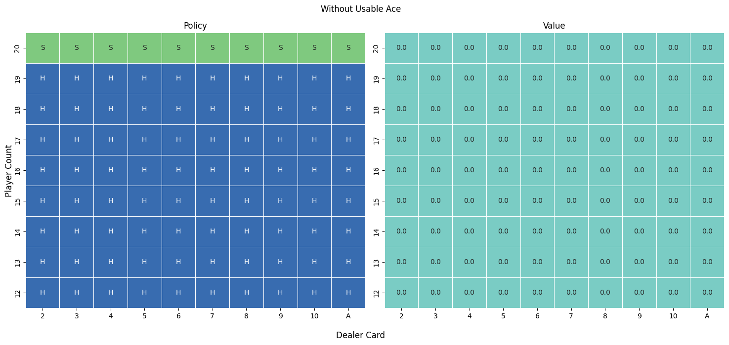
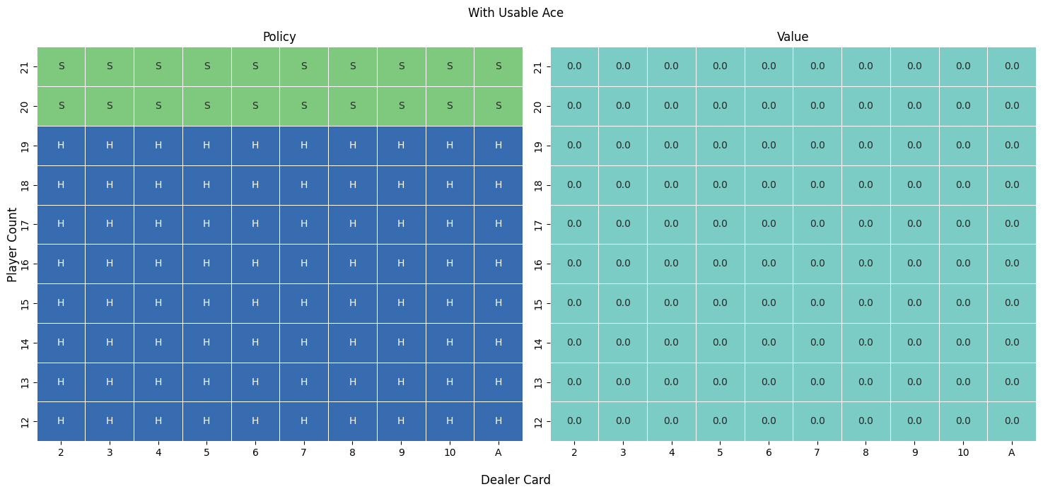
Sutton & Barto also suggest an initial policy for the example. For the initial policy, the player hits any hard (no usable ace) or soft (contains usable ace) hand up a total of 20 and then stands. Figure 1 and Figure 2 depict this initial policies in a format similar to how basic strategy is often displayed. The value matrix is also initialized to zero.
Policy Convergence
In order to know how many episodes are necessary to arrive at the optimal policy, we need some measure of convergance. For this example I decided to look at two different measures. The first is the RMSE from the difference between the value matrices at checkpoints. When the policy is changing a lot at the beginning, the value matrix will also change and register a larger RMSE. The second is a count of the number of policy changes from one snapshot to the next. As the policy converges, this number will be zero.
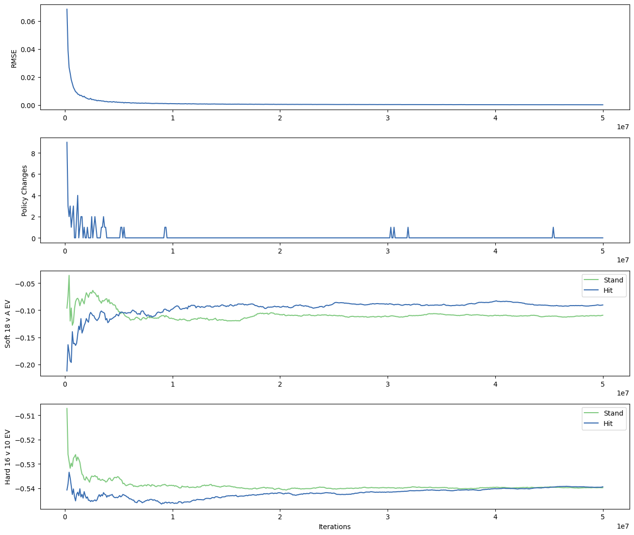
With the implementation I used, the basic strategy policy appeared converged after 50 million episodes. This took about 4 minutes to run. One challenge is that the EV values calculated by MC simulations are only estimates of the actual values. Because they come from random sampling, the values never completely stabilize. For some hands the difference in EV between hitting and standing is very small, so the policy can flip back and forth between these values while converging. An example of such a hand shown in Figure 3 is the soft 18 against a dealer ace. After 50 million episodes, the difference in EV was -0.109 for a stand and -0.090 for a hit. Both actions lose, but hitting loses slightly less often.
“Basic Strategy” Policy
To generate a strategy card from our MC ES we can select the action that has the highest EV for each state. Figure 4 and Figure 5 match the results presented in Example 5.3 of Sutton & Barto.
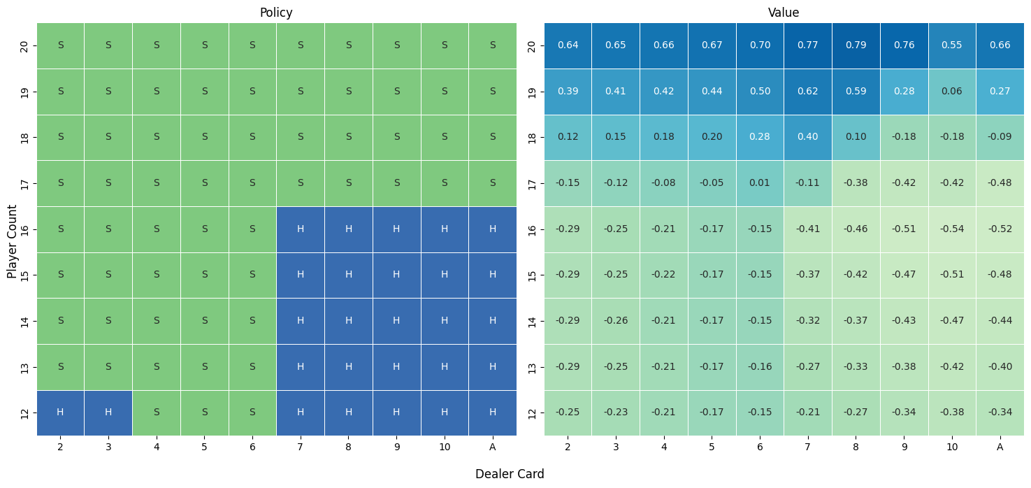
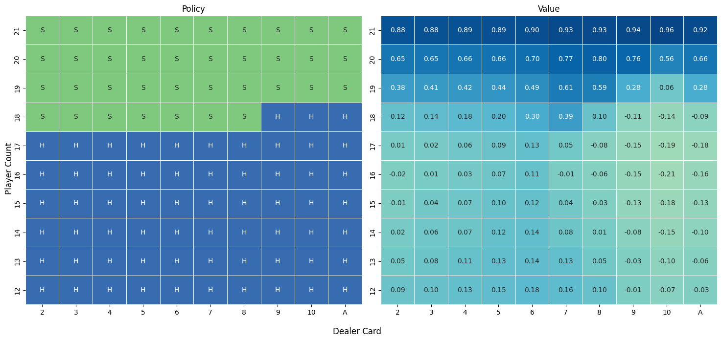
Sutton & Barto do point out that the policy derived from this exercise is almost the same as Thorp’s 1966 basic strategy.
This policy is the same as the “basic” strategy of Thorp (1966) with the sole exception of the leftmost notch in the policy for a usable ace, which is not present in Thorp’s strategy. We are uncertain of the reason for this discrepancy, but confident that what is shown here is indeed the optimal policy for the version of blackjack we have described.
The “notch” is the soft 18 versus dealer ace that we discussed as an edge case and is show in Figure 3. There are a few possible reasons that Sutton & Barto might have come up with different policy for that hand. The simplest would be that more episodes were required for policy stability, but given the reputation of the authors I suspect they were highly cognizant of convergence requirements. The more likely answer is a subtle difference in the way the deck was modeled, which I will discuss in the next article.
A second way to look at the policy is in terms of regret from not choosing the best action.
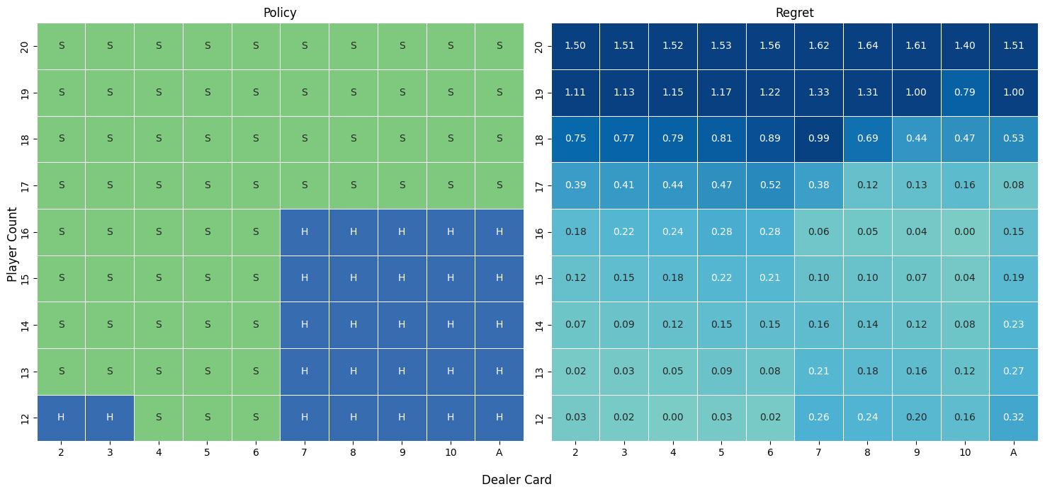
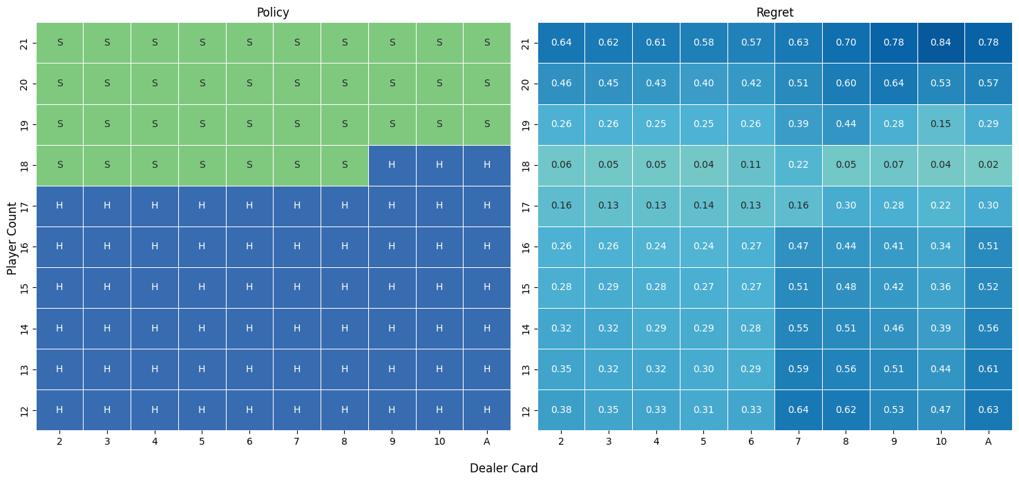
Figure 6 and Figure 7 show how close to a tossup some of the choices are. For example, the difference between hitting and standing on a hard 16 against a dealer 10 is probably too small to measure after 50 million episodes. We can also see this in the convergence plot Figure 3.