Efficiently Solving Equations with Tridiagonal Matrices
Benchmarking Python implementations across algorithms
The implementations generated for this study are now available as a standalone python library called tridiag.
Summary
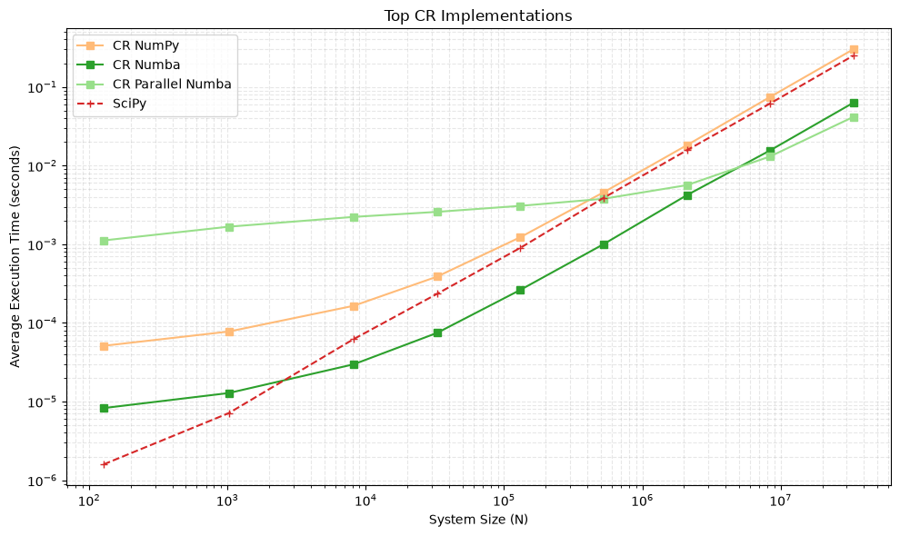
In this article we compare performance of several different implementations of a tridiagonal matrix system solver. These implementations include the Thomas Algorithm, Cyclic Reduction, and Parallel Cyclic Reduction. Where possible, the algorithms are implemented to utilize multi-core parallelization. We found that our Numba implementation of cyclic reduction outperformed the industry standard SciPy solver (Virtanen et al. 2020) even on a single core as the system size exceeded \(10^4\) rows.
Introduction
Tridiagonal matrices arise frequently in many fields of engineering and science, particularly when solving partial differential equations using finite difference methods. When a one-dimensional problem is discretized, the resulting system of linear equations often has a tridiagonal matrix structure, where each variable only depends on its immediate neighbors.
A classic example of this is the modeling of heat transfer in biological tissue. In Bioheat Transfer Modeling, we saw how the discretization of the Pennes Bioheat Equation using the Crank-Nicholson method leads to a system that can be efficiently solved using specialized algorithms.
In this article we implement several different algorithms for solving systems with tridiagonal matrices and benchmark their performance when given access to sequential and parallel compute architectures.
Problem Definition
A tridiagonal matrix is a square matrix \(A\) of size \(N \times N\) where all non-zero elements are confined to the main diagonal, the sub-diagonal (directly below the main diagonal), and the super-diagonal (directly above the main diagonal).
A tridiagonal linear system is of the form \(Ax = d\), which can be expressed as a set of equations for \(i = 0, \dots, N-1\):
\[ a_i x_{i-1} + b_i x_i + c_i x_{i+1} = d_i \tag{1}\]
where: - \(b_i\) are the elements of the main diagonal. - \(a_i\) are the elements of the sub-diagonal (\(a_0\) is usually defined as 0 or ignored). - \(c_i\) are the elements of the super-diagonal (\(c_{N-1}\) is usually defined as 0 or ignored).
Overview of Algorithms
Solving this system efficiently is crucial for large-scale simulations, as general-purpose solvers (like Gaussian elimination) would take \(O(N^3)\) operations, whereas specialized tridiagonal solvers can achieve the same result in \(O(N)\) operations.
The Thomas Algorithm, also known as the Tridiagonal Matrix Algorithm (TDMA), is a simplified form of Gaussian elimination specifically designed for tridiagonal linear systems of equations. Its efficiency stems from exploiting the sparse structure of tridiagonal matrices, leading to a much faster solution than general Gaussian elimination, \(O(N)\) operations compared to \(O(N^3)\). It is a direct and sequential method first described by Llewellyn Thomas (Thomas 1949). For a detailed explanation and derivation of this algorithm, please see Thomas Algorithm.
Cyclic Reduction (CR) is another direct method for solving tridiagonal linear systems of equations. Unlike the Thomas algorithm, which is inherently sequential, CR repeatedly transforms the original system into a smaller system of the same form. Developed by Hockney (Hockney 1965), this reduction process continues until the system becomes small enough to be solved directly, after which the eliminated unknowns are recovered through a back-substitution phase. The reduction phase is suitable for parallel computing architectures as it utilizes simultaneously eliminating odd- or even-indexed unknowns. For a detailed explanation and derivation of this algorithm, please see Cyclic Reduction.
Parallel Cyclic Reduction (PCR) is a variation of the CR algorithm designed for maximum parallelism. While standard CR reduces the system size by half at each step and requires a sequential upsweep (back-substitution) phase, PCR eliminates the upsweep phase entirely (Hockney and Jesshope 1981). For a detailed explanation and derivation of this algorithm, please see Parallel Cyclic Reduction.
Work Complexity and Total Steps
The relationship between work complexity and total steps (depth) can be a fundamental trade-off in algorithm design. The best tradeoff frequently depends on whether the algorithm can utilize parallel computation from multiple CPU cores or a GPU.
- Work Complexity: The total number of operations performed.
- Total Steps: The minimum amount of time required to finish if you had an infinite parallelization. This represents the longest chain of sequential dependencies.
| Feature | TDMA | CR | PCR |
|---|---|---|---|
| Total Steps | \(2N\) (Sequential) | \(2 \log_2 N\) (Parallel) | \(\log_2 N\) (Parallel) |
| Work Complexity | \(O(N)\) | \(O(N)\) | \(O(N \log_2 N)\) |
| Parallelism | all sequential | Parallel steps, sequential phases | all parallel |
With TDMA there is no opportunity for parallelizing the work. You can’t add more processing cores to make it go faster because each task needs to wait for the previous one to finish. CR achieves parallel speedup without significantly increasing the total amount of work. By halving the problem size at each step, we’ve compressed the sequential chain of \(N\) steps into a tree of \(\log N\) levels. The total work stays \(O(N)\) because the number of active workers decreases as the problem gets smaller (\(N \to N/2 \to N/4 \dots\)). PCR does more work in order to support more parallelization. It actually performs redundant operations by calculating information across all rows in each step to avoid the back-substitution phase used in CR.
Performance Expectations
As \(N\) increases, the performance relationship between these three algorithms changes dramatically depending on whether we are using a single core or multiple cores.
Consider the formula for execution time:
\[ T \approx \frac{\text{W}}{\text{P}} + \text{S} \tag{2}\]
where \(W\) is work, \(P\) is number of processors, and \(S\) is steps. Using our values from the table above we can estimate the following:
\[ \begin{aligned} T_{TDMA} &\approx \frac{N}{P} + N \\ T_{CR} &\approx \frac{N}{P} + \log N \\ T_{PCR} &\approx \frac{N \log N}{P} + \log N \end{aligned} \tag{3}\]
Parallelism only helps us reduce the \(\frac{W}{P}\) part of the equation. It can never make the \(S\) part go away. That is why we choose algorithms with \(\log N\) steps for parallel hardware, even if they do more total work.
Benchmark Results
To benchmark the performance of each implementation, we built a tool to generate random tridiagonal matrix systems of arbitrary size with known solutions. We could then test the average time to solve the system multiple trials of each implementation. For implementations that required just in time compliation, we allowed for a warmup run to perform the JIT. Therefore, these benchmarks do not include the compilation time. For a solving a single system, this would increase the time to solve significantly for those implementations. However, we elected to omit that time since the most likely application of these algorithms would be solving a large number of systems over the dimension of time or space.
As a point of comparison we also included SciPy’s LAPACK-based solver as a reference. Specifically we used scipy.linalg.solve_banded, which wraps LAPACK’s dgtsv. This is the industry standard for sequential CPU performance, written in highly optimized Fortran.
Benchmark calculations were performed on an Apple M5 Macbook Pro with 10 cores (4 super, 6 efficiency). We tested across tridiagonal system sizes from \(N=10^2\) to \(N=10^8\) revealing several critical insights into algorithm choice and modern hardware limits.
Sequential
In cases where only a single compute core is available, the most optimized sequential algorithms should win. TDMA does the fewest total calculations and should be fastest.
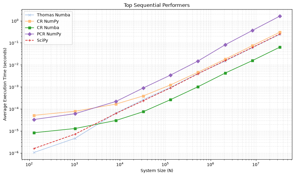
At small \(N\) the JIT version of the TDMA algorithm is by far the fastest, as expected. Across all tested \(N\), it performs very comparably to the reference SciPy LAPACK solver. If we next look at the NumPy implementations of CR and PCR, we see that NumPy CR is slower than Thomas but faster than NumPy PCR across most of the range. This is also expected since CR is doing more calculations than TDMA but fewer than PCR.
However, there are also some surprising results. First, we see that the fastest implementation when \(N > 10^4\) is Numba CR. This is a JIT version of standard CR algorithm that does not use prange parallelization. Without parallelization, how does the CR beat TDMA when it does more calculations. The answer almost certainly lies in LLVM’s ability to vectorize operations and utilize the SIMD capabilities of the hardware. SIMD is a type of parallelization that allows single core machines to perform the same operation on different data simultaneously. LLVM is smart enough to use this automatically when compiling and running the CR algorithm, giving it parallel-like performance on a single core.
This also explains the second surprising result. The NumPy CR implementation performance approaches the performance of the Numba TDMA and SciPy TDMA algorithms at larger \(N\). Again, this shouldn’t be possible since CR is doing more operations than TDMA. However, NumPy can also utilize vectorized operations due to its built in support of SIMD and our implementation is built to support this. The benchmarks show that SIMD is able to close the performance gap between CR and a highly optimized sequential implementations even though it is doing more calculations in total.
The last question is then, why does CR Numba perform better than CR NumPy if both implementations can utilize SIMD? One possible explanation is that NumPy uses pre-compiled C and Fortan binaries that may not be able to fully utilize the capabilities of the hardware. LLVM may be able to detect and utilize the specific SIMD sets on the hardware when compiling, adding up tp a bit of extra performance.
Parallel
Based on the performance boost we saw in the sequential results from SIMD, utilizing multi-core parallelization should give us even better results. As \(P\) increases in Equation 2, we start to see a tradeoff between work and number of steps. If \(P\) is sufficiently large, the time term becomes dominated by the steps. For TDMA, this approaches \(N\) and for CR and PCR it approaches \(\log N\). We would expect CR and PCR to outperform TDMA when we utilize parallelization.
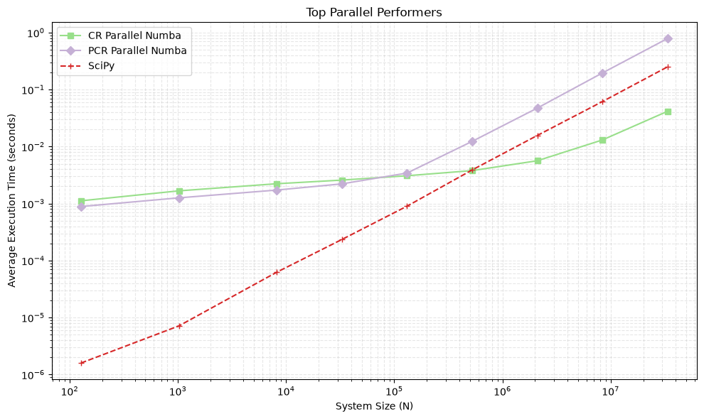
Somewhat surprisingly, the parallel implementations are consistently slower than the SciPy (and Numba TDMA) implementations up system sizes of about \(10^6\). With the number of cores available on our computer, the overhead of sychronizing memory and moving data appears to negate the benefits of parallelization until \(N\) gets quite large.
At very large values of \(N\), the parallel Numba CR implementation is clearly the fastest, about an order of magnitude faster than the benchmark SciPy implementation.
Combined Benchmark Results
Figure 3 below shows benchmark results for all implementations we tested. Unsurprisingly, the pure python implementations that used regular loops were not competitive with the more optimized versions. The reference SciPy implementation is quite fast and remains an excellent default choice. However, the Numba TDMA implementation is slightly faster at smaller \(N\) and the CR Numba implementation is significantly faster at larger \(N\). For the largest values of \(N\) tested, the CR Parallel Numba implementation is the fastest. For practitioners looking to maximize tridiagonal system solving throughput, these are options worth considering. However, this may be hardware dependent and it’s worth testing on more platforms.
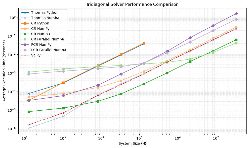
The CR algorithm seems to be the best “all around” solution on the hardware we used. Specifically, the sequential Numba implementation of CR which utilizes the SIMD vectorization is fast across a wide range of \(N\). In fact, it’s a significant performance boost over the reference SciPy implementation for most of the system sizes we tested.